Weka thread I have found that questions are answered very promptly and there is a lot of activity at the site, so you don't have to wait a long time to get a response. In addition there are some great books put out by Ian Witten and Eibe Frank that guide you through the practical data mining with a minimal barrage of mathematical theory:
Data Mining Practical Machine Learning Tools and Techniques With Java Implementations I have the first edition and have found it an immensely useful reference.
There are a variety of built in learning modules included in the free utility (Weka), such as linear regression, neural networks (a.k.a multilayer perceptrons), decision trees, support vector machines, and even genetic algorithms.
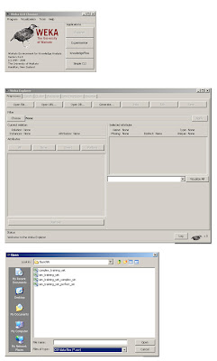
Fig 1. Using the Weka Gui
In Fig 1., we see the Weka GUI Chooser has been opened and the Explorer option was selected. The native format that Weka commonly uses is the .ARFF format, fortunately for us, however, it also reads in .CSV files, which are easily created with a save option in excel. The excel file we will first train is sim_training_set_perfect_sin.csv. Once loaded, you will see all of the relevant variables in the Weka Explorer shell.
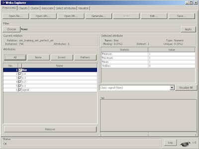
Fig 2. Loaded Excel csv training source file for Weka
We notice some new variables have been introduced that were not in part 1.
To understand why, let's show the CSV file that is used here.
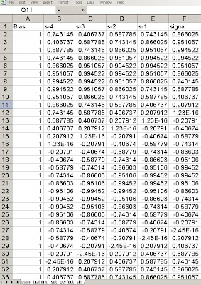
Fig 3. Training set variables.
What we see is that the original perfect sine wave signal has been preserved in the column labeled signal. The additional signals, s-1, s-2, s-3, s-4 are often called delayed or embedded (dimension) variables. They are simply lagged values of the signal that are used to train the neural network. There is no exact method to determine the number of lagged values, although a number of different methods exist. For now, we will simply accept that four delayed values of the signal are useful. The last column, called bias, is common to neural networks. The bias node allows the neural network to shift the constant signal input to the network via training. For instance, imagine our signal had an average of 2.0 but we were learning it. The neural network needs to have some input that will track that constant value or it will have large offset errors that will obstruct convergence. The bias node accomplishes that operation. Those familiar with Engineering theory will recognize this node as a DC bias.
Ok, so once other thing we notice in the GUI interface is the Class:signal(num) is selected on the bottom right. This is because we are predicting a numerical class, rather than a nominal one (which is the typical default for classification schemes).
Next, we select the classify tab to select our learning scheme, which in this case will be the MultilayerPerceptron.
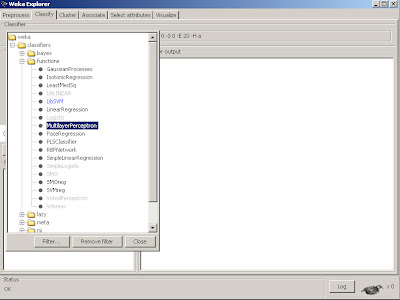
We then want to make sure certain options are selected.
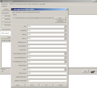
We set nominalToBinaryFilter and normalize attributes as False, as we don't wish to modify the input data to be binary and are not using nominal attributes. However, we
want the normalizeNumericClass set to True as mentioned earlier, it will force the normalization scheme to be set to Weka's internal limiting range, so we don't have to. Also, we will train for 1000 epochs.
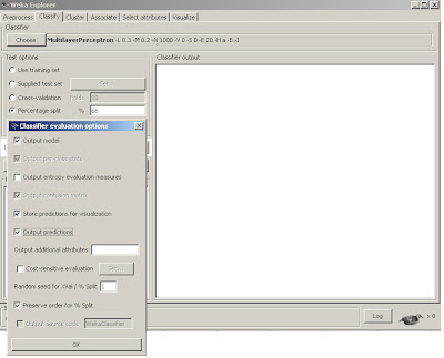
Fig 6. Preferences for MLP training model.
We will build a model by training on 66% of the data. We want to store and output the predictions so that we can visually see what they look like. Lastly, we will Preserve order for split as it allows us to display the predicted out of sample time series in the original order. With all of these features set, we simply click OK and the start button and it will quickly build our first Neural Network model!
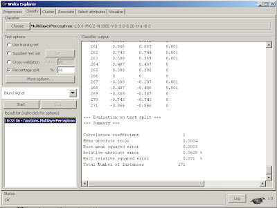
Fig 7. Results with summary of statistics console.
If we scroll up we can see the actual weights that the model converged upon for our Multilayer Perceptron that will be used to predict the out of sample data.
We can see that there is a nice printout of the last 34% of results (271 out of sample data points) along with the predicted value and error, as well as a useful summary of statistics in the bottom of the console. We often use Root mean squared error as a performance metric for neural net regressions. In this case, the number .0005 is quite good. But let's use a little trick to get a visual inspection of just how good. We can actually grab the data from the console (by selecting it with the left mouse button and dragging), then copy this data back into excel. As a result, we can then plot the actual versus predicted out of sample results inside of excel.
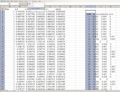
Fig 8. Importing prediction results back into Excel.
Notice that we cut and paste the data from the Weka console back into Excel, but must select text to columns in order to separate the data back into columns.
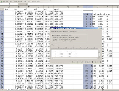
Fig 9. Selecting the regions to separate as columns.
And tada! We can now plot the predicted vs. actual values. And look how nicely they line up. The errors are extremely small on the out of sample set, notice some are 0, others are .001, imperceptible to the eye, without zooming way in on that point.
It actually found a perfect model for this time series (we will expand a bit later why), and the errors can be attributed to numerical precision.
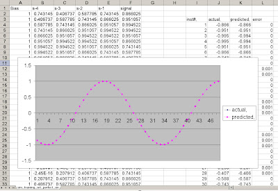
Fig 10. Resulting plot of predicted vs. actual data.
We have now just built a basic Neural Network with a simple sine wave time series using Weka and Excel. The predicted out of sample results were extremely good.
However, as we will see, the data signal we used, the simple sine wave is a very easy signal to learn as it is perfectly repetitive and stationary. We will see that as the signal gets increasingly complex, the prediction results do not work as well.
That's it for Part 2, comments are welcome.


